Dynamometer for High-Speed, Low-Torque Motors

This post details the design and construction of an absorption dynamometer for small, high-speed, low-torque motors. It was completed by mechanical engineering seniors Sina Atalay, Arda Gençgel, and Hümeyra Kayadibi at Boğaziçi University in January 2023.

We summarize dynamometer types, outline project specs, compare absorption unit options, and justify our choice of dynamic braking. The system is modeled in state-space, tuned to meet constraints, and simulated in MATLAB (code on GitHub). Finally, we show the assembled device and sample measurements.

Introduction

Dynamometers measure either the torque and speed produced by a rotating prime mover (e.g., an internal combustion engine) or the torque and speed required to drive a device (e.g, a pump). They fall into two main categories:

• Absorption Dynamometer: Applies a load to a rotating test device and measures its output torque and speed.
• Motoring Dynamometer: Drives a test device and measures the required input torque and speed.

Absorption dynamometers are essential for characterizing a motor’s torque–speed and power curves, especially when supplier data is unreliable or unavailable.

Specifications

We required a low-cost absorption dynamometer for testing high-speed, low-torque motors at Boğaziçi University, with the following targets:

• Speeds up to 20,000 RPM
• Power dissipation up to 80 W

Key design questions included:

1. What type of absorption unit?

   Measuring power requires braking and dissipation energy. Therefore, the test motor’s output energy must be absorbed by the dynamometer for measurement.

2. How to measure torque?

3. How to measure speed?

4. Should we control speed and/or torque?

   Dynamometers are typically used to assess motor performance at various speeds and torques. Therefore, the user may need to control speed, torque, or both.

Absorption Unit Selection

Dynamometers apply a braking load to the test motor, causing energy dissipation according to:

$$\begin{equation} \text{Power} = (\text{Torque}) \cdot (\text{Rotation Speed}) \end{equation}$$

Common braking methods include mechanical friction, hydraulic brakes, and eddy current brakes.

Another approach is to couple a second DC motor (the load motor) to the test motor. The load motor then operates as a generator, absorbing the test motor’s energy output. This type of dynamometer is called an electric dynamometer¹, and it was selected for this project.

Before selecting the absorption method, the available options were researched and evaluated. The final decision considered constraints on time, budget, available technology, and design requirements. This section outlines the absorption unit options and the rationale for selecting an electric dynamometer.

Mechanical Friction Brake

The simplest mechanical braking method is a Prony brake (Figure 1²), which both absorbs the test motor’s energy and measures torque. It is also simple to build.

As shown in Figure 1, a lever is clamped to the shaft, and the load $F$ is measured. The load $F$ is carried by the frictional force between the shaft and the lever. The torque is then calculated using statics:

$$\begin{equation} \text{Torque} = Fl \end{equation}$$

where $l$ is the distance between the point where load $F$ is applied and the center of the motor’s shaft.

Load $F$ can be measured using a weight or a load cell. Figure 2³ shows a Prony brake dynamometer with a load cell.

While a Prony brake is affordable and easy to build, controlling the load or speed is difficult and very hard to automate electronically. Load adjustments must be made manually, and brake pads require regular replacement.

Eddy Current Brake

When a metal moves through a magnetic field, circulating eddy currents are induced. According to Lenz’s law, these currents generate opposing magnetic fields, producing a force that resists motion⁴. Many braking systems use this effect.

An eddy current dynamometer typically uses a metal disk attached to a shaft and a controllable magnetic field (Figure 3⁵). Eddy currents in the rotating disk produce braking, with the braking force controlled by moving magnets or adjusting current in electromagnets. The energy is dissipated as heat due to the disk’s electrical resistance.

While eddy current braking allows for controllable load, accurately measuring torque is difficult. Designing a well-balanced disk for high-speed shafts also poses mechanical challenges.

Dynamic Brake

When an electric motor is coupled to the test motor and then operated as a generator (load motor), it produces opposing torque. This is called dynamic braking. Electric dynamometers use this method to convert the test motor’s mechanical energy into electrical power, which can be dissipated as heat or returned to the supply.

Advantages include:

• DC motors are widely available and easily used as generators.
• No mechanical wear, resulting in longer lifespan than friction systems.
• Torque is easily calculated from generator current due to the linear torque-current relationship in DC motors.
• Rotational speed is easily calculated from generator voltage due to the linear speed-voltage relationship in DC motors.
• Load can be varied by adjusting electrical resistance.
• Absorbed energy can potentially be reused.
• The system can be adapted to function as a motoring dynamometer.

The main drawback is that braking torque depends on rotational speed, making low-speed braking difficult (discussed further in the Theory section).

The Decision

Given our time and equipment constraints, the eddy current brake was rejected as the most difficult to build and maintain, offering no unique advantages.

We gathered detailed information on Prony and dynamic brakes and reviewed their implementations. Ultimately, we chose dynamic braking and built an electric dynamometer. Its ease of use, electronic controllability, and potential for future upgrades made it the better choice.

Theory

To understand how the load motor generates torque to resist rotation, we first need to review the basics of a DC motor.

Basics of a DC Motor

A basic DC motor model is shown in Figure 4⁶.

Two fundamental principles govern the operation of a DC motor.

First principle: Faraday’s law of induction states that as the coil rotates, the changing magnetic flux induces a voltage difference between the terminals⁴. This induced voltage, called the electromotive force (EMF), is expressed by Equation 3:

$$\begin{equation} V=K_V\omega \end{equation}$$

where $K_V$ is the EMF constant of the motor, $\omega$ is the angular speed of the shaft, and $V$ is the induced voltage⁷.

Second principle: When current flows through the coil, a magnetic torque is exerted on the rotor. The generated torque is given by:

$$\begin{equation} T=K_T i \end{equation}$$

where $K_T$ is the torque constant of the motor, $i$ is the coil current, and $T$ is the generated torque⁷.

Result: When the motor’s rotor is rotated, it generates EMF. If the motor terminals are connected, the EMF causes current to flow. This current produces a torque that resists motion, following Lenz’s Law⁴. The dynamometer’s load motor operates on this mechanism.

Formulation and Design Variables

To further analyze and optimize the dynamometer’s design, the system was modeled. The schematic is shown in Figure 5.

When the test motor starts to rotate, the load motor also rotates. This generates a voltage difference between the load motor’s terminals (per Equation 3), and current $i_l$ begins to flow (per Equation 4). This current causes braking.

A voltmeter and ammeter will be used to measure speed and torque, as shown in Figure 5. Torque and speed can be calculated using Equations 3 and 4, but the values of $K_{V,l}$ and $K_{T,l}$ must be known. How these are determined is explained in the Load Motor Selection section.

All symbols used in Figure 5 are described in Table 1.

Symbol	Description
$V$	Voltage sensor measurement
$i_l$	Current sensor measurement
$\omega$	Angular velocity
$T$	Torque
$R$	Potentiometer’s resistance
$V_\text{in}$	Test motor’s voltage input
$R_t$	Test motor’s internal resistance
$L_t$	Test motor’s internal inductance
$K_{V,t}$	Test motor’s back EMF constant
$K_{T,t}$	Torque constant of the test motor
$i_t$	Current that flows through the test motor
$R_l$	Internal resistance of the load motor
$L_l$	Internal inductance of the load motor
$K_{V,l}$	Back EMF constant of the load motor
$K_{T,l}$	Torque constant of the load motor
$i_l$	Current that flows through the load motor

The fundamental independent design variables are:

• $K_{V,l}$, $K_\text{T,l}$, $L_l$, $R_l$: determined by the load motor selection
• $R$: determined by the potentiometer selection

We will analyze the system to select the best values for these variables to meet the design targets.

Steady State Analysis and Measurement Range

The selected load motor and potentiometer range determine the dynamometer’s measurement range. To find this range, we assume the system is in a steady state ($\dot{i}_l = 0$), so inductances do not affect the equations. Using Kirchhoff’s voltage law⁸ and Equation 3:

$$\begin{equation} i_l(R_l+R)-K_{V,l}\omega=0 \end{equation}$$

Using Equation 4 for the load motor gives:

$$\begin{equation} i_l=\frac{T}{K_{T,l}} \end{equation}$$

Combining Equations 5 and 6:

$$\begin{equation} T(R,\, \omega)=\frac{\omega K_{T,l} K_{V,l}}{R+R_l} \end{equation}$$

Combining Equation 1 with Equation 7:

$$\begin{equation} P(R,\, \omega)=\frac{\omega^2 K_{T,l} K_{V,l}}{R+R_l} \end{equation}$$

where $P$ is the power.

Equations 7 and 8 highlight two key points about electric dynamometers:

1. As $R + R_l \to 0$, $T \to \infty$. In practice, this means the load motor’s shaft would become impossible to rotate if $R + R_l$ were zero. Therefore, $R + R_l$ must be greater than zero and determines the maximum braking torque at a given $\omega$.
2. As $\omega$ decreases, both $T$ and $P$ decrease. This makes measuring low-speed, high-torque motors difficult without using a gear reducer.

Another factor limiting the measurement range is the power absorption limit. In this design, the test motor’s power output is dissipated as heat by the resistors $R$ and $R_l$. These resistors have a maximum power dissipation capacity, denoted as $P_\text{lim}$:

$$\begin{equation} \frac{\omega^2 K_{T,l} K_{V,l}}{R+R_l}<P_\text{lim} \end{equation}$$

Equations 7, 8, and 9 together define the dynamometer’s measurement range. The load motor must be selected to satisfy these design criteria.

Transient State Analysis

In the previous section, we assumed the system was in steady state, so the motors’ internal inductance did not affect the equations. However, the transient state is also critical because the dynamometer’s response time to changes in the potentiometer’s resistance can impact ease of use.

Figure 5 should be examined closely to model the dynamometer mathematically. The system’s mathematical model is required for simulation.

Applying Kirchhoff’s voltage law and using Equation 3, we obtain:

$$\begin{equation} V_\text{in}-R_t i_t - L_t \dot{i}_ t - \omega K_\text{V,t}=0 \end{equation}$$ $$\begin{equation} (R+R_l)i_l-L_l\dot{i}_l-\omega K _\text{V,l}=0 \end{equation}$$

Assuming both motors have effective rotational inertia $I$ and viscous damping $c$, the torque balance equation using Equation 4 becomes:

$$\begin{equation} i_tK_\text{T,t}-I\dot{\omega}-c\omega-i_l K_\text{T,l}=0 \end{equation}$$

Combining Equations 10, 11, and 12, and expressing them in state-space form:

$$\begin{equation} \begin{bmatrix} \dot{i _ t } \\\\ \dot{\omega} \\\\ \dot{i _ l } \end{bmatrix} = \begin{bmatrix} {-R} _ t/L _ t & {-K} _ \text{V,t}/L _ t & 0 \\\\ K _ \text{T,t} /I & -c/I & -{nK} _ {T,l} /I \\\\ 0 & {nK} _ \text{V,l} /L _ l & (-R(t)-R _ l)/L _ l \end{bmatrix} \begin{bmatrix} i_t \\\\ \omega \\\\ i_l \end{bmatrix} + \begin{bmatrix} 1/L_ t \\\\ 0\\\\ 0 \end{bmatrix} \begin{bmatrix} V_ {\text{in}} \end{bmatrix} \end{equation}$$

The dynamometer can be simulated using a computational tool by solving Equation 13. A MATLAB code was developed to solve this system and simulate the dynamometer. The code is available on GitHub.

Load Motor Selection

The most crucial part of designing an electric dynamometer is selecting the load motor. The load motor determines $K_{V,l}$, $K_{T,l}$, and $R_l$, which in turn define the dynamometer’s measurement range, as shown in Equations 7, 8, and 9.

Considering the operational limits discussed in the Specifications section (maximum speed of 20,000 RPM and power of 80 W), we searched local shops for a suitable DC motor. We specifically looked for motors with cooling fans, since the test motor’s energy output would be dissipated as heat in the load motor circuit. Eventually, we found and purchased an old motor without any specifications, shown in Figure 6.

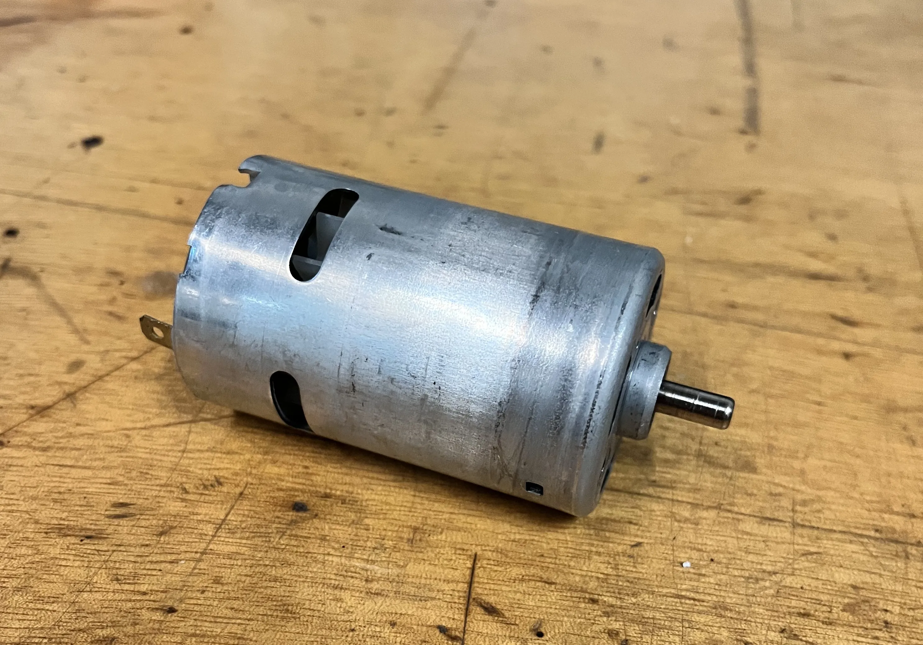
The only way to determine if this motor was suitable was to measure $K_{V,l}$, $K_{T,l}$, and $R_l$, then use the relevant equations to calculate the measurement range. The selected motor turned out to be a good fit for our design. The measurement methods and results are explained in the following sections.

EMF Constant Measurement

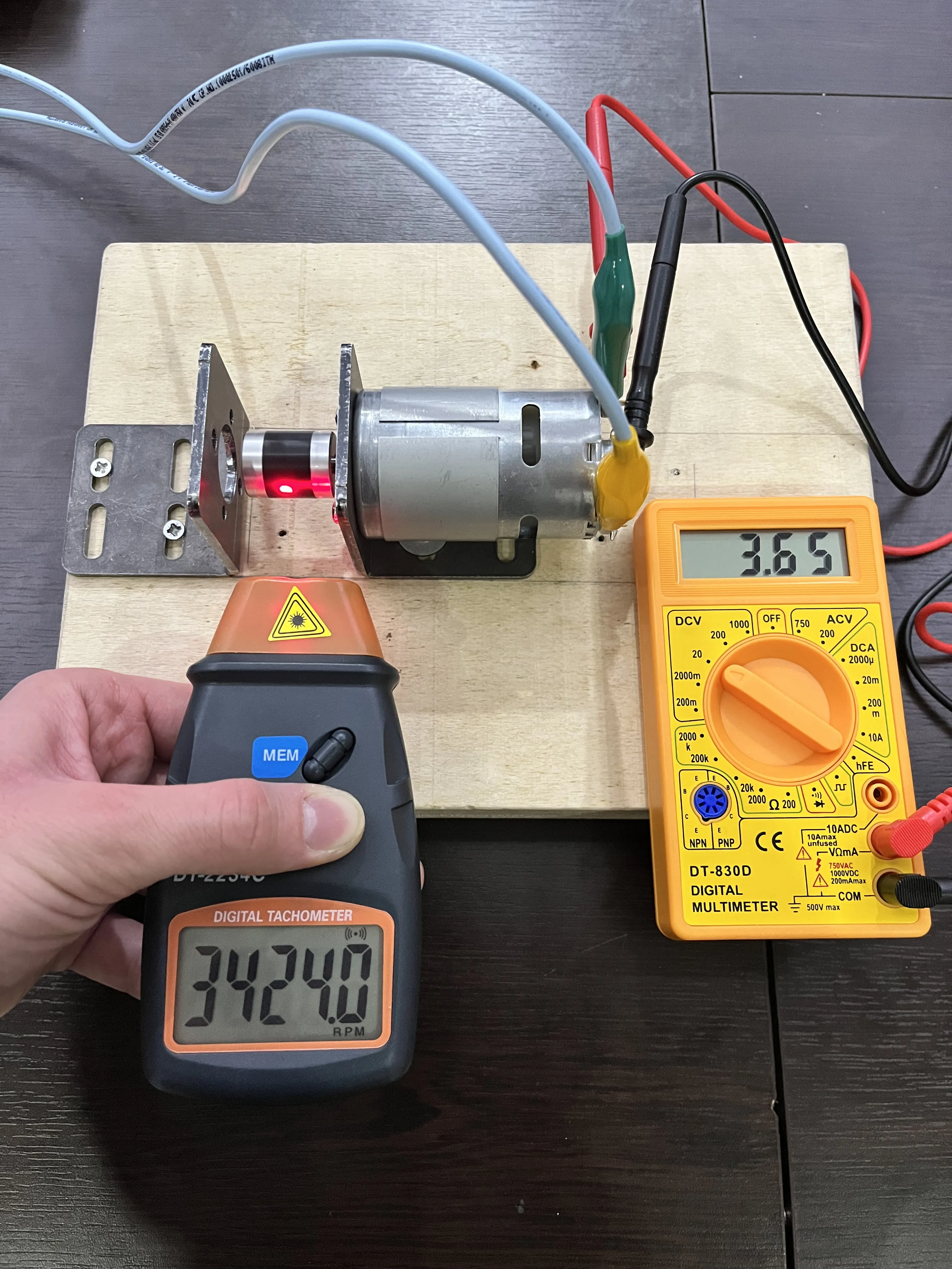
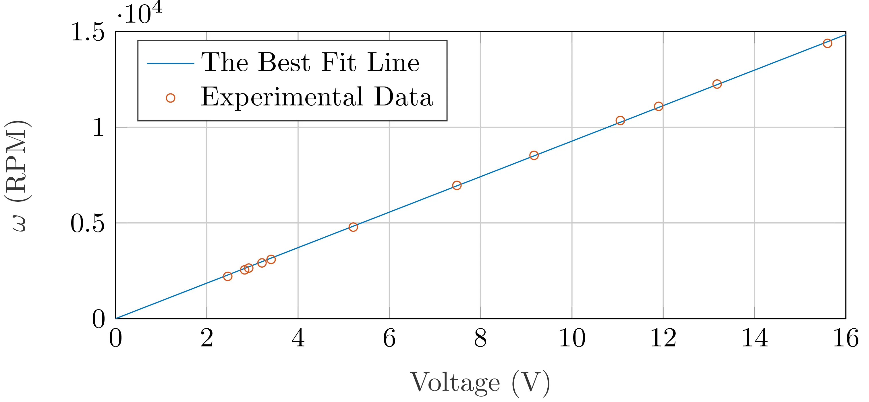
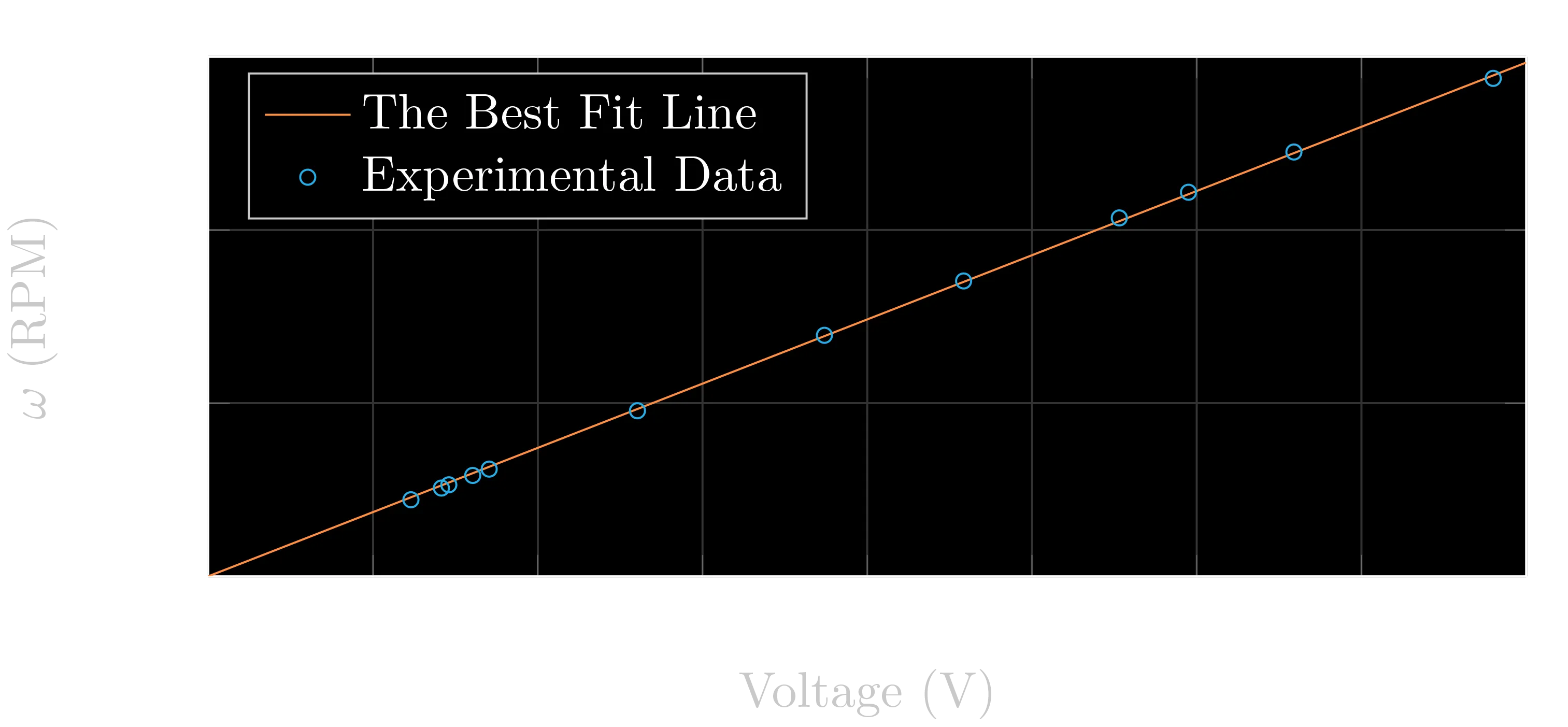
As explained in Basics of a DC Motor section and Equation 3, the voltage difference between a DC motor’s terminals is linearly proportional to its speed through the EMF constant, $K_{V,l}$.

To determine $K_{V,l}$, we applied different voltages to the motor and measured the corresponding rotational speeds, as shown in Figure 7. The measurement data are listed in Table 2.

Voltage (V)	$\omega$ (RPM)
2.46	2210
2.83	2548
2.92	2642
3.21	2912
3.41	3095
5.21	4781
7.48	6960
9.17	8529
11.06	10350
11.90	11091
13.18	12253
15.60	14380

The data were then fitted using Equation 3. The data points and regression line are shown in Figure 8. The EMF constant $K_{V,l}$ was found to be $0.0103\, (\text{V}\cdot\text{s})/\text{rad}$.

Torque Constant Measurement

Similarly, the current flowing through a DC motor is linearly proportional to the torque it generates, through the torque constant $K_{T,l}$, as shown in Equation 4.

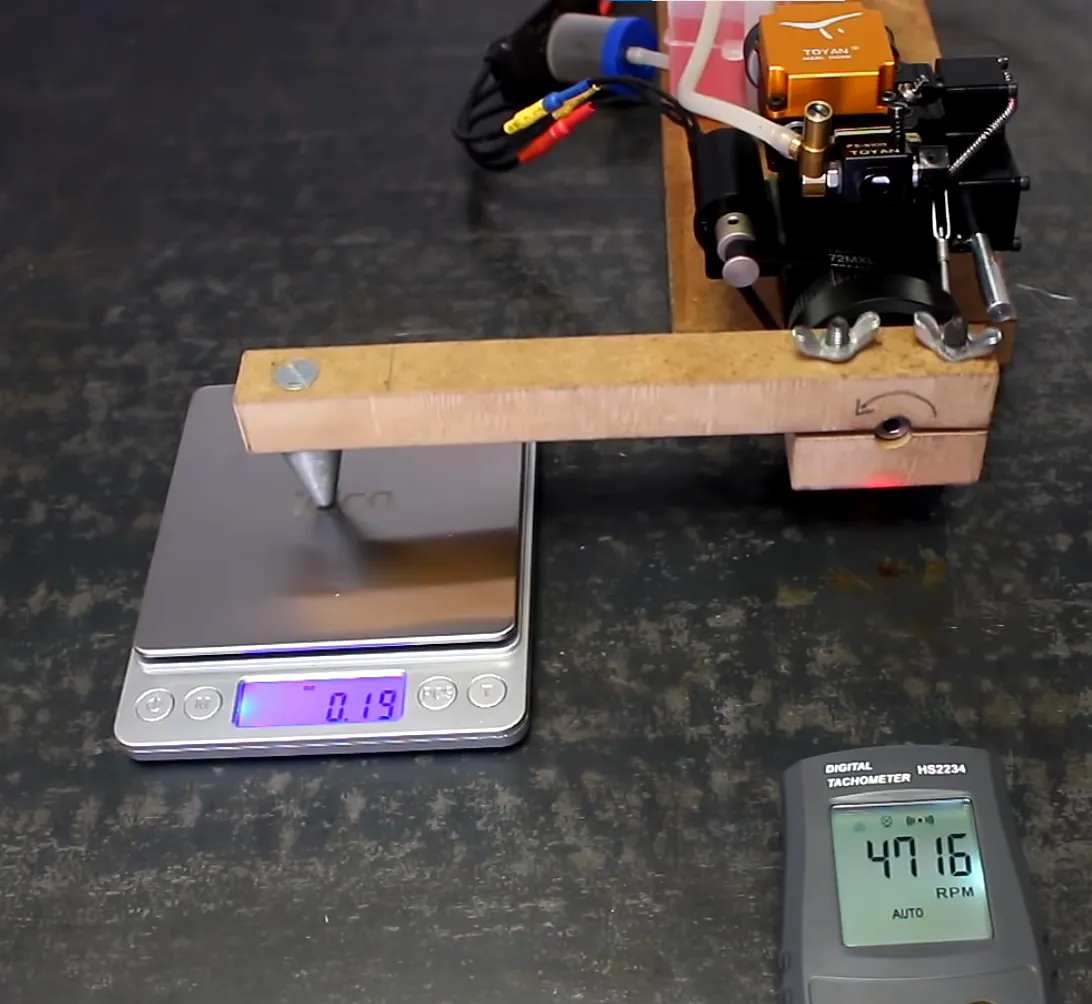
We supplied different currents to the motor and measured the corresponding torque. However, measuring torque was more complex than measuring speed. First, we attached a lightweight tool to the shaft and powered the motor. The tool was chosen so the motor could not lift it fully but could displace it at a measurable angle. For each supplied current, we measured the angular displacement of the tool, as shown in Figures 9, 10, and 11.

Next, we located the tool’s center of mass and measured its weight using a precision scale. Finally, we calculated the torque from the angle data using statics.

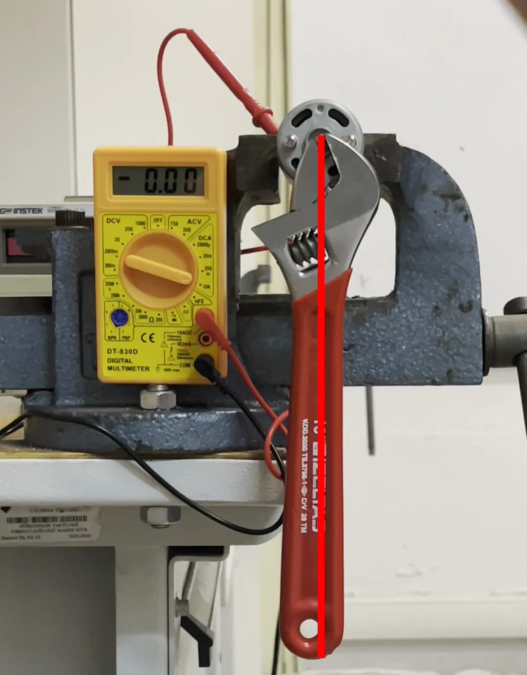
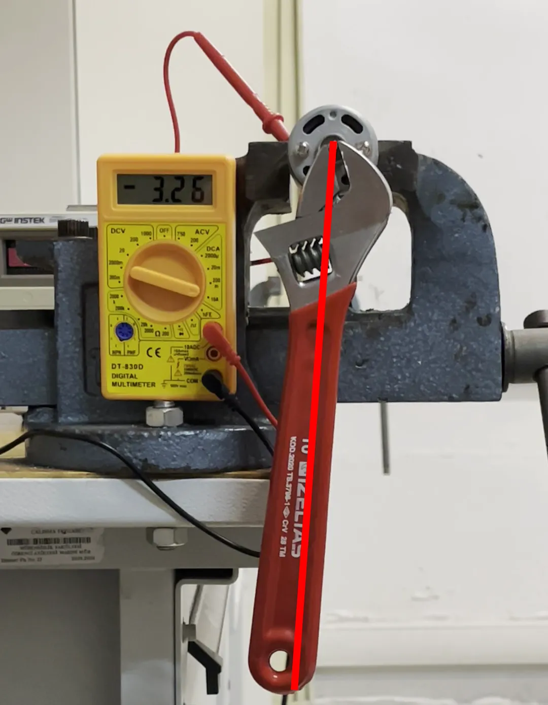
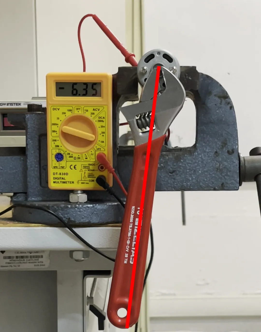
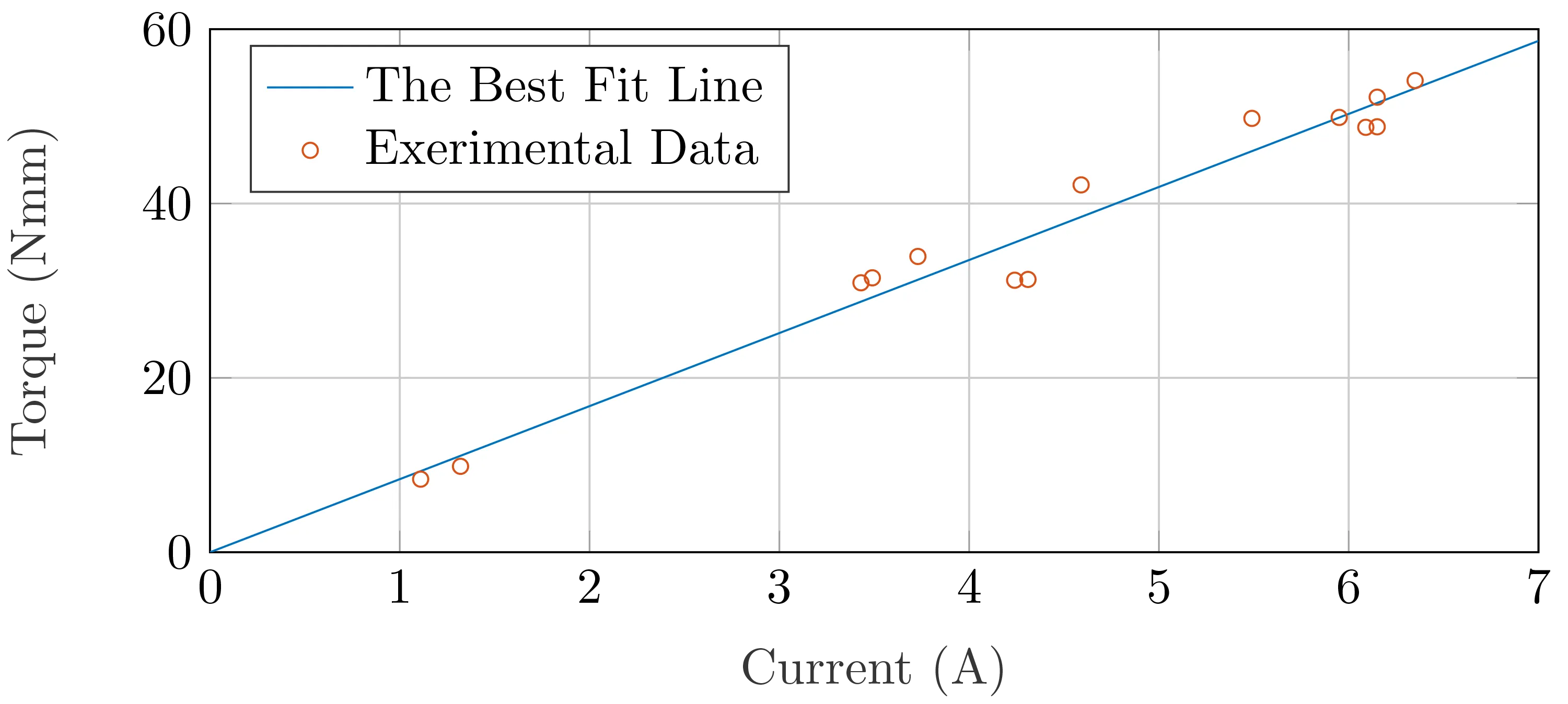
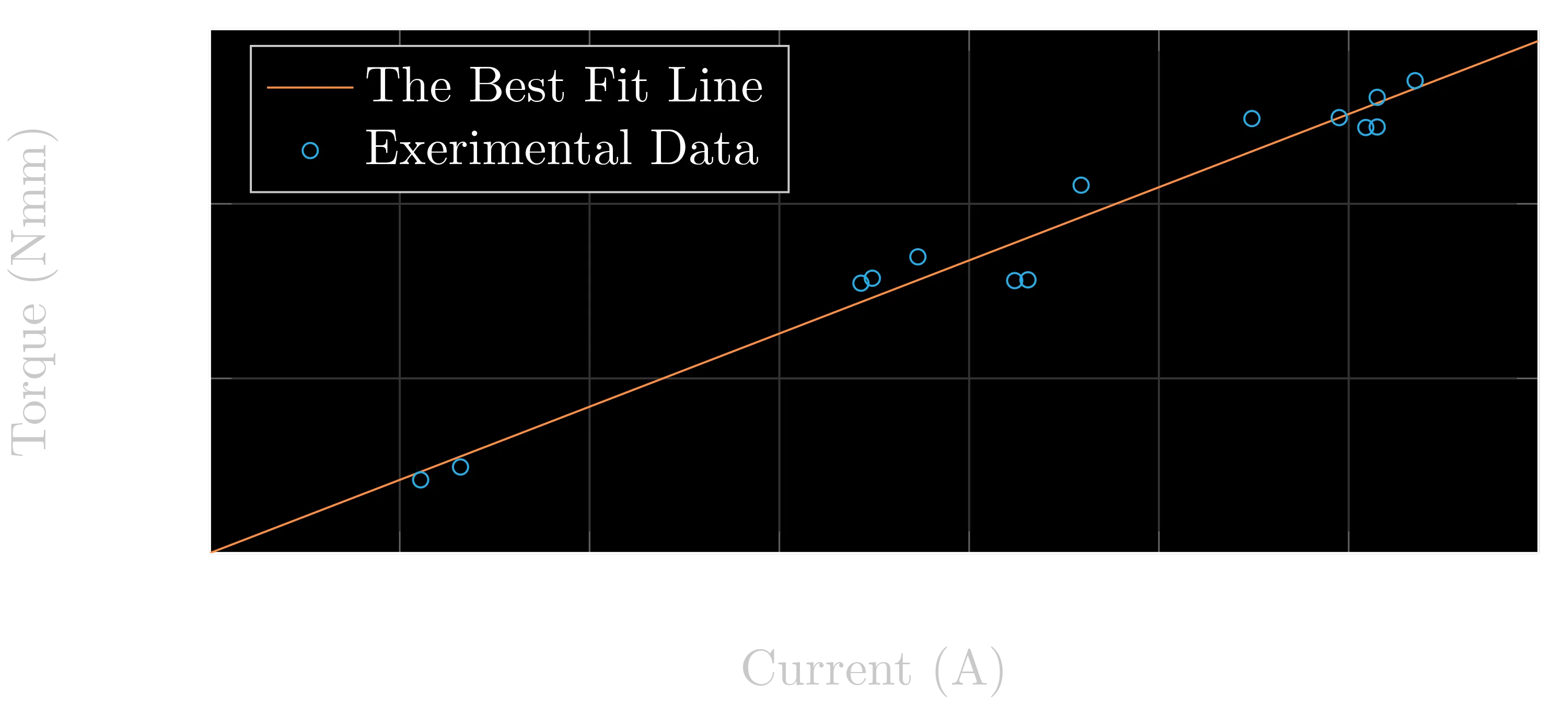
Table 3 shows the measured currents and calculated torque values. The data were fitted using Equation 4. The data points and regression line are plotted in Figure 12. The torque constant $K_{T,l}$ was found to be $0.00840\, (\text{N}\cdot\text{m})/\text{A}$.

Current (A)	Torque (Nmm)
1.11	8.4
1.32	9.9
3.43	30.9
3.49	31.5
3.73	33.9
4.24	31.2
4.31	31.3
4.59	42.1
5.49	49.8
5.95	49.9
6.09	48.7
6.15	48.8
6.15	52.2
6.35	54.1

Internal Resistance Measurement

Measuring the internal resistance of a DC motor is straightforward. We powered the motor, stopped the shaft using an external tool, and divided the voltage across the terminals by the current. Since $\omega = 0$, the armature does not contribute to the terminal voltage, so the only contribution comes from internal resistance. The result was: $R_l=8.75\, \mathrm{V}/2.13 \, \mathrm{A}=4.11 \,\Omega$.

Measurement Range

With all required parameters now determined, the dynamometer’s measurement range (operation range) can be calculated.

As shown in Equations 7 and 8, torque and power are functions of $R$ and $\omega$. These equations define the maximum measurable torque and power at a given rotation speed. Maximum values occur when $R = 0$. Note that $R$ can be increased up to $\infty$, which corresponds to disconnecting the load motor’s terminals.

$$\begin{equation} T_{\text{max}}(\omega)=\frac{\omega K_{T,l} K_{V,l}}{R_l} \end{equation}$$ $$\begin{equation} P_{\text{max}}(\omega)=\frac{\omega^2 K_{T,l} K_{V,l}}{R_l} \end{equation}$$

Equations 14, 15, and the power limit $P_\text{lim} = 100, \mathrm{W}$ are graphed in Figure 13. The blue region shows the dynamometer’s measurement range.

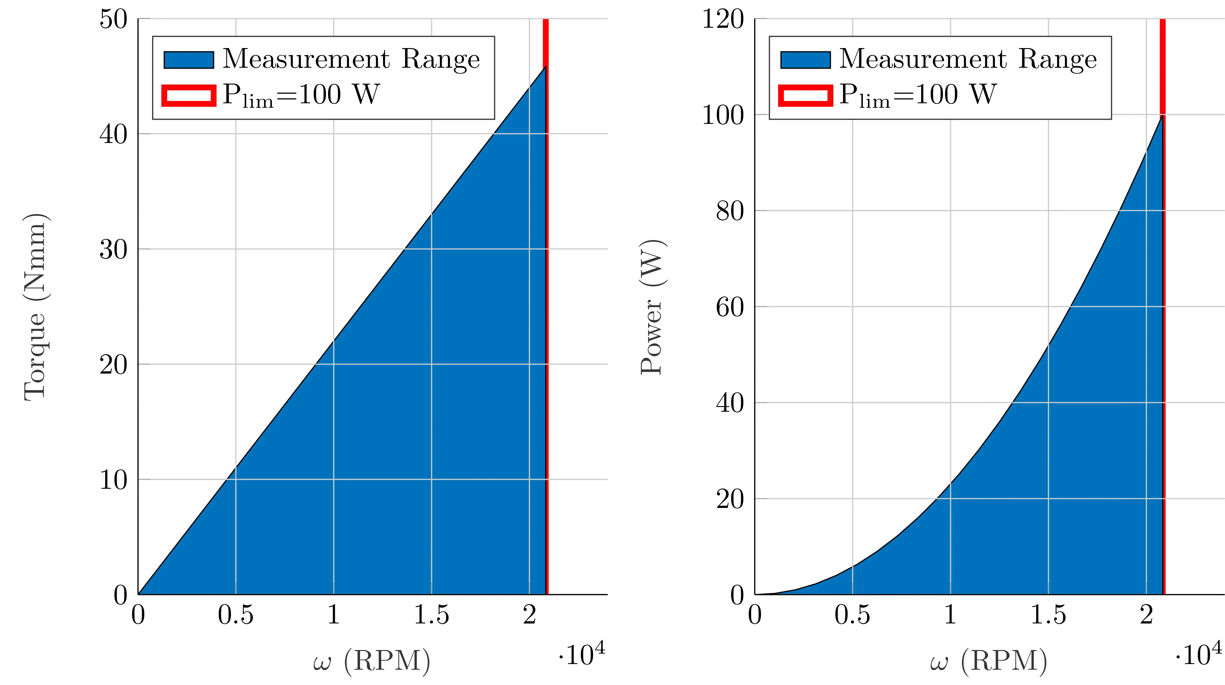
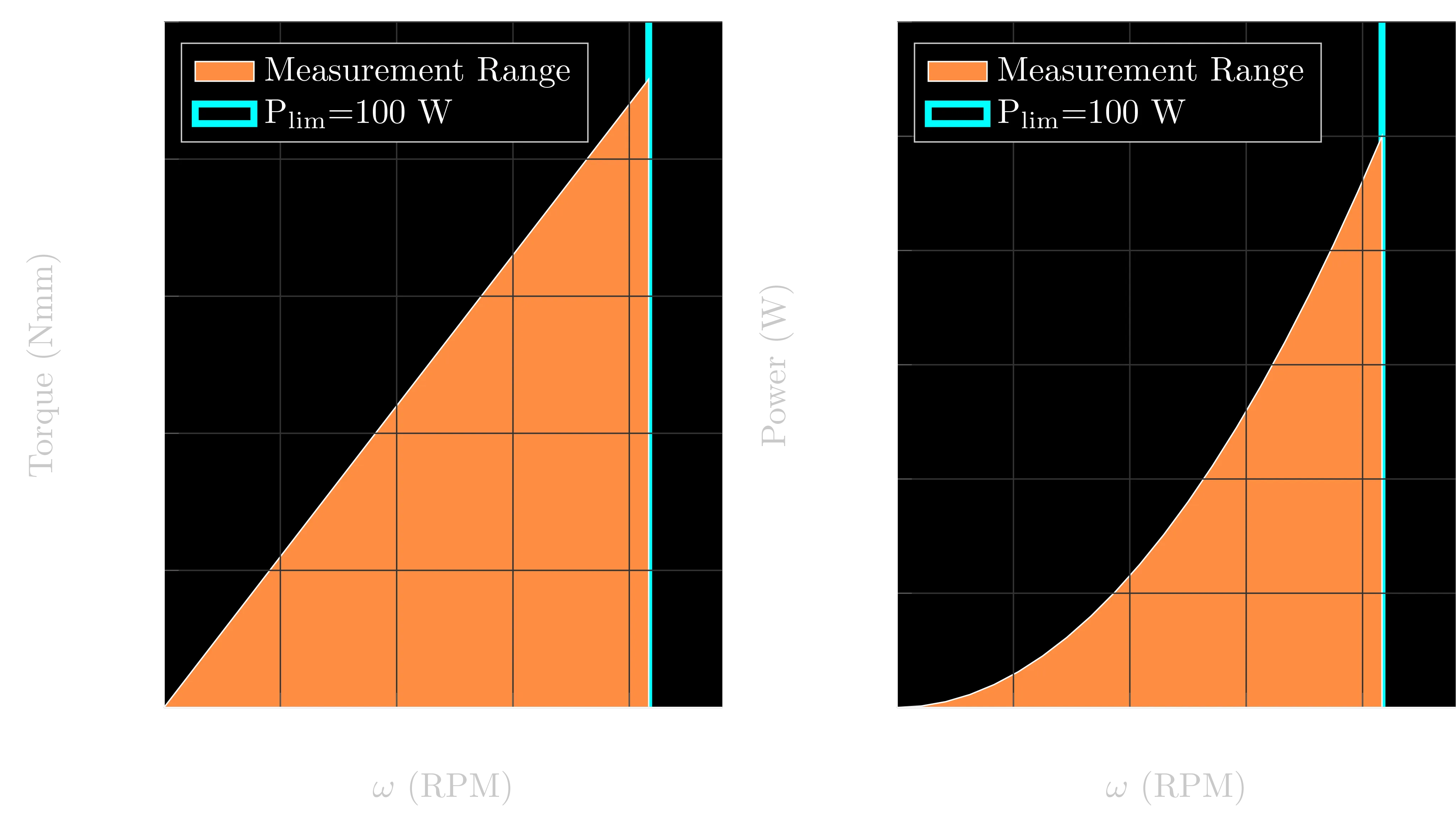
The results show the dynamometer can operate at speeds up to 20,000 RPM and power up to 80 W. Therefore, the selected load motor is suitable. However, the maximum braking torque decreases as rotation speed decreases. As a result, this design is only suitable for high-speed, low-torque motors. A gear reducer could be used to increase speed and reduce torque for motors outside this range.

Uncertainty Analysis

The uncertainty in the dynamometer’s measurements depends on the accuracy of the voltage sensor, current sensor, $K_{V,l}$, $K_{T,l}$, and $R_l$. Torque and rotational speed are calculated from the voltage and current sensor values using the equations below:

$$\begin{equation} \omega=\frac{V+i_lR_l}{K_{V,l}} \end{equation}$$ $$\begin{equation} T=K_{T,l}i_l \end{equation}$$

The uncertainties of $K_{V,l}$, $K_{T,l}$, $R_l$, $V$, and $i_l$ contribute to the combined uncertainty of $\omega$ and $T$. Recall that the most probable estimate of the combined uncertainty of a quantity $A$, which depends on variables $x_1, \cdots, x_n$, is:

$$\begin{equation} U_A=\sqrt{\left(\left.\frac{\partial A}{\partial x_1}\right| _ {x=\overline{x}} U_{x_1}\right)^2 + \left(\left.\frac{\partial A}{\partial x _ 2}\right| _ {x=\overline{x}} U _ {x_2}\right)^2 + \cdots + \left(\left.\frac{\partial A}{\partial x_n}\right|_{x=\overline{x}} U _ {x_n}\right)^2 } \end{equation}$$

where $\overline{x}$ is the average value of $x$, and $U_{x_i}$ is the uncertainty of $x_i$⁹.

Applying Equation 18 to the measurements of $T$ and $\omega$:

$$\begin{equation} \begin{split} U_\omega&=\sqrt{\left(\frac{1}{K_{V,l}}U_V\right)^2+\left(\frac{R_l}{K_{V,l}}U_{i_l}\right)^2+\left(\frac{\overline{i_l}}{K_{V,l}}U_{R_l}\right)^2+\left(\frac{\overline{V}+\overline{i_l}R_l}{K_{V,l}^2}U_{K_{V,l}}\right)^2} \\\\ &=206.13\,\text{RPM} \end{split} \end{equation}$$ $$\begin{equation} \begin{split} U_T&=\sqrt{\left(K_{T,l} U_{i_l}\right)^2+\left(\overline{i_l} U_{K_{T,l}}\right)^2} \\\\ &=1.51\,\mathrm{N}\cdot\mathrm{mm} \end{split} \end{equation}$$

Here, $\overline{i_l}$ and $\overline{V}$ are assumed to be 2.5 A and 5 V, respectively.

The uncertainties in $K_{V,l}$ and $K_{T,l}$ were calculated as follows:

$$\begin{equation} \begin{split} U_{K_{V,l}}&=\frac{\sum\limits^{n} _ {n=1} \left|V_n/\omega_n-K _ {V,l}\right|}{n} \\\\ &=0.0001\,\mathrm{V}\cdot\mathrm{s}/\mathrm{rad} \end{split} \end{equation}$$ $$\begin{equation} \begin{split} U_{K _ {T,l}}&=\frac{\sum\limits^{n} _ {n=1} \left|T_n/i_n-K_{T,l}\right|}{n} \\\\ &=0.00006\,\mathrm{N}\cdot\mathrm{m}/\mathrm{A} \end{split} \end{equation}$$

The uncertainties from the measurement devices are given in Table 4:

Variable	Uncertainty
$V$	0.01 V
$i_l$	0.01 A
$R_l$	0.01 Ω

The uncertainties calculated in Equations 19 and 20 define the precision of the dynamometer.

Building the Dynamometer

After selecting the load motor and determining the theoretical measurement range, the next step was to build the dynamometer. This section summarizes the dynamometer’s general workflow, as well as the mechanical and electronic designs.

Workflow

The dynamometer’s workflow is shown in the block diagram in Figure 14.

The load and speed are controlled by adjusting the potentiometer resistance ($R$). The user can easily change the resistance, which adjusts the braking load and motor speed, as described by Equations 7 and 8. As the user changes the resistance, the electronic circuit continuously collects measurement data.

A potentiometer is an accessible and simple component. We purchased one from a local shop rated for up to 100 W with a resistance range from $0$ to $80 \, \Omega$. This was a suitable choice given the power limit set by the design criteria.

Mechanical Design and Components

Before building the electronic measurement circuit, the mechanical system was designed and assembled using two DC motors (a test motor and a load motor). The final product and its 3D CAD model are shown in Figures 15 and 16.

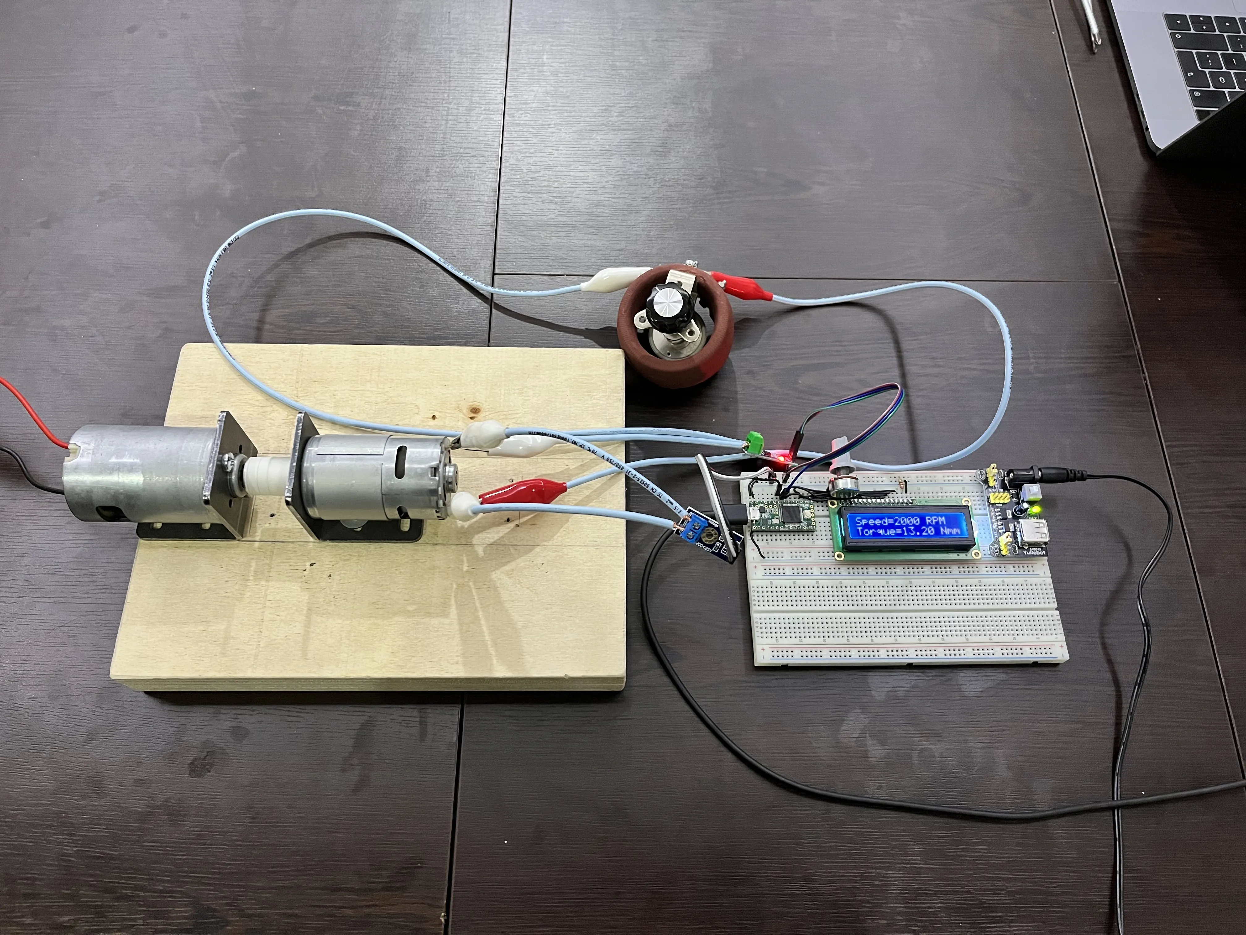
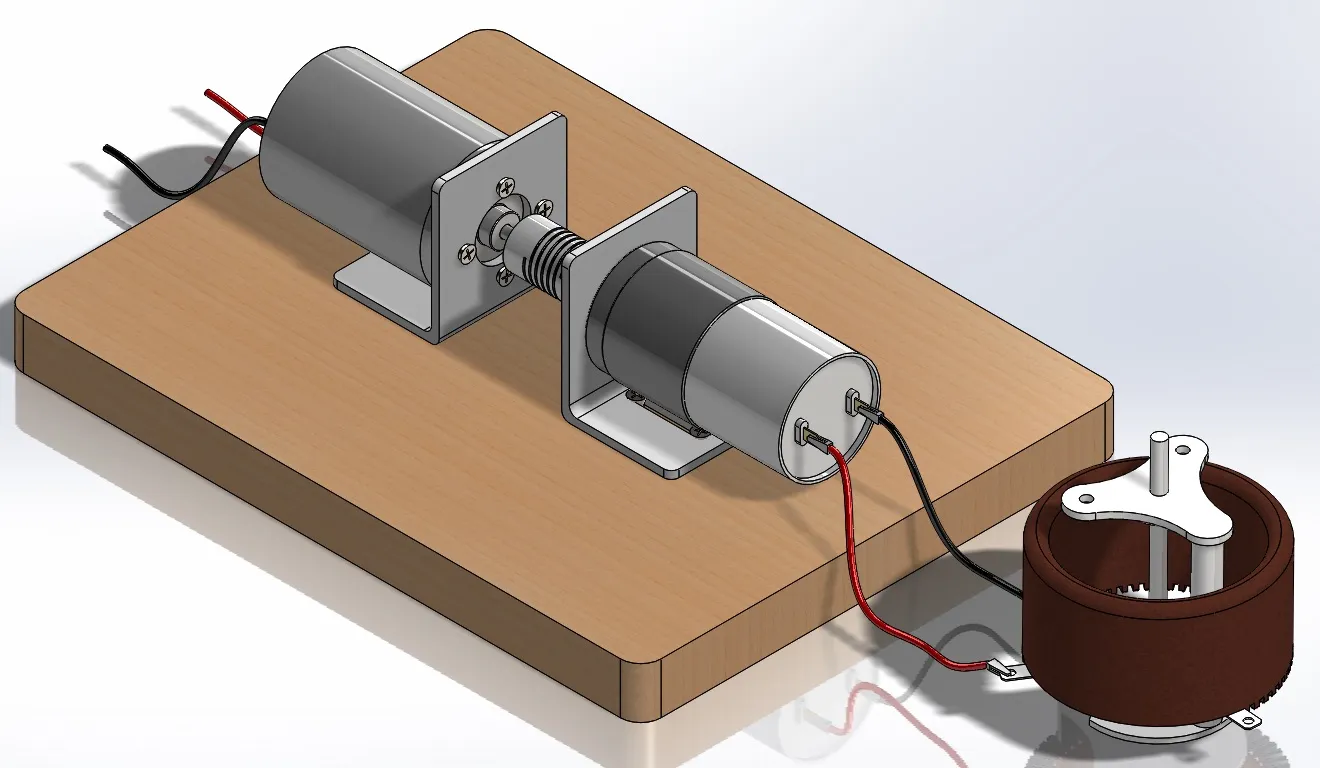
The mechanical assembly includes the following components:

• A wooden block serving as the base.
• Two DC motor mounts for the load and test motors.
• A flexible coupling to connect the shafts of the test motor and load motor.
• A potentiometer to control the braking torque.

The mechanical assembly process was straightforward:

1. The motor mounts were positioned on the wooden base and fastened with screws.
2. The motors were secured to the mounts and coupled together.
3. The potentiometer was attached to the load motor.
4. The electronic system was connected to the load motor and potentiometer.

Electronic Design and Components

After the mechanical assembly, the next step was to design the electronic circuit and program a microcontroller to take and collect measurements. The final circuit schematic is shown in Figure 17. The key design considerations were:

• A current sensor was required.
• A voltage sensor was required.
• An LCD screen was needed for users without a computer.
• MATLAB integration should be possible.
• Measurement accuracy should be as high as possible.

We used a basic Arduino-like microcontroller, the Teensy 3.2¹⁰. The programming focused on two main objectives:

1. Reducing sensor noise.
2. Integrating with MATLAB.

Both sensors’ outputs were sampled 20 times per second. The mean of these samples was used as the measurement value to reduce noise. As a result, the dynamometer produced one data point per second.

Integration with MATLAB was provided via a USB connection. However, connecting to a computer is not necessary for basic operation because the system includes an LCD screen.

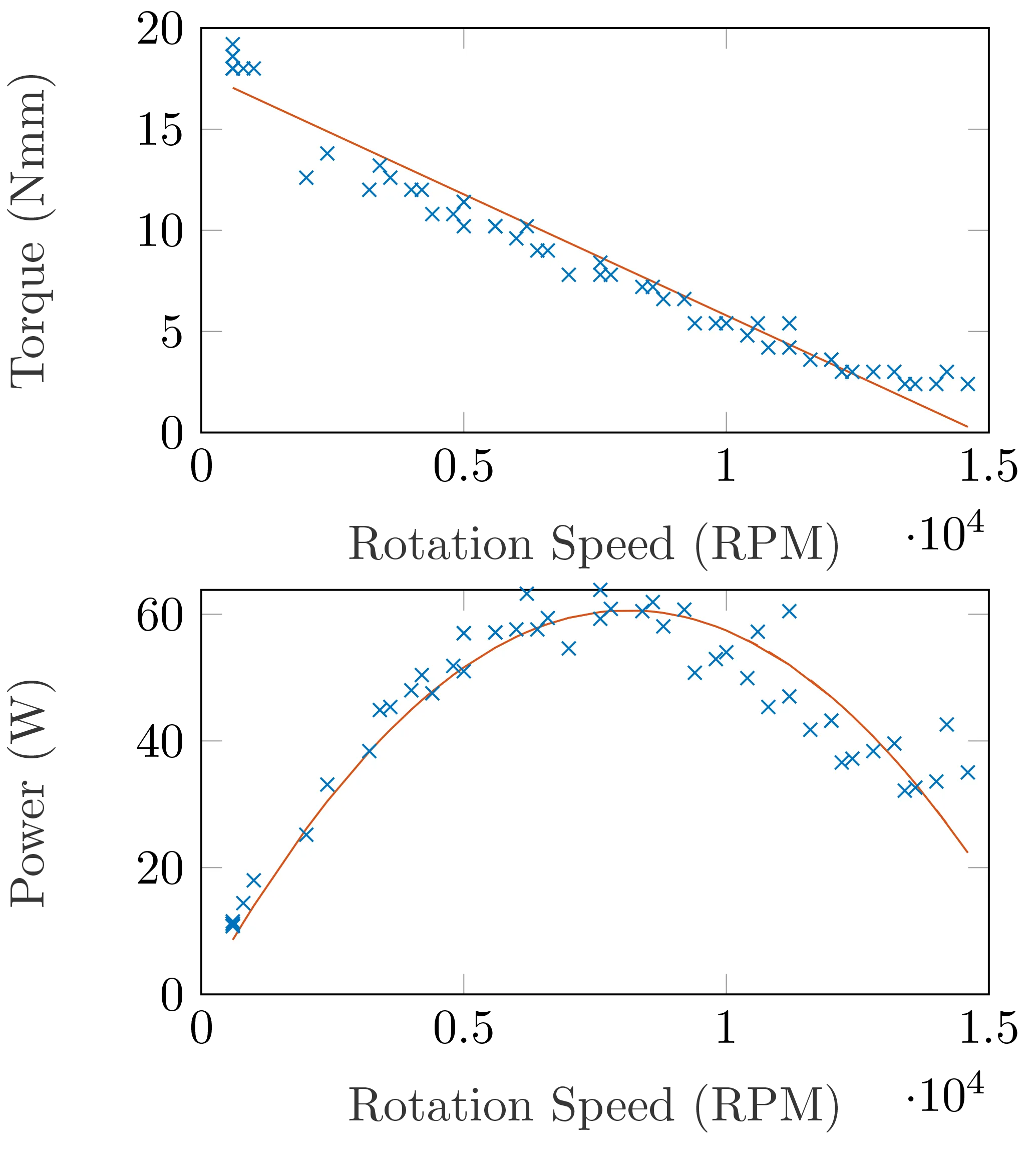
Results

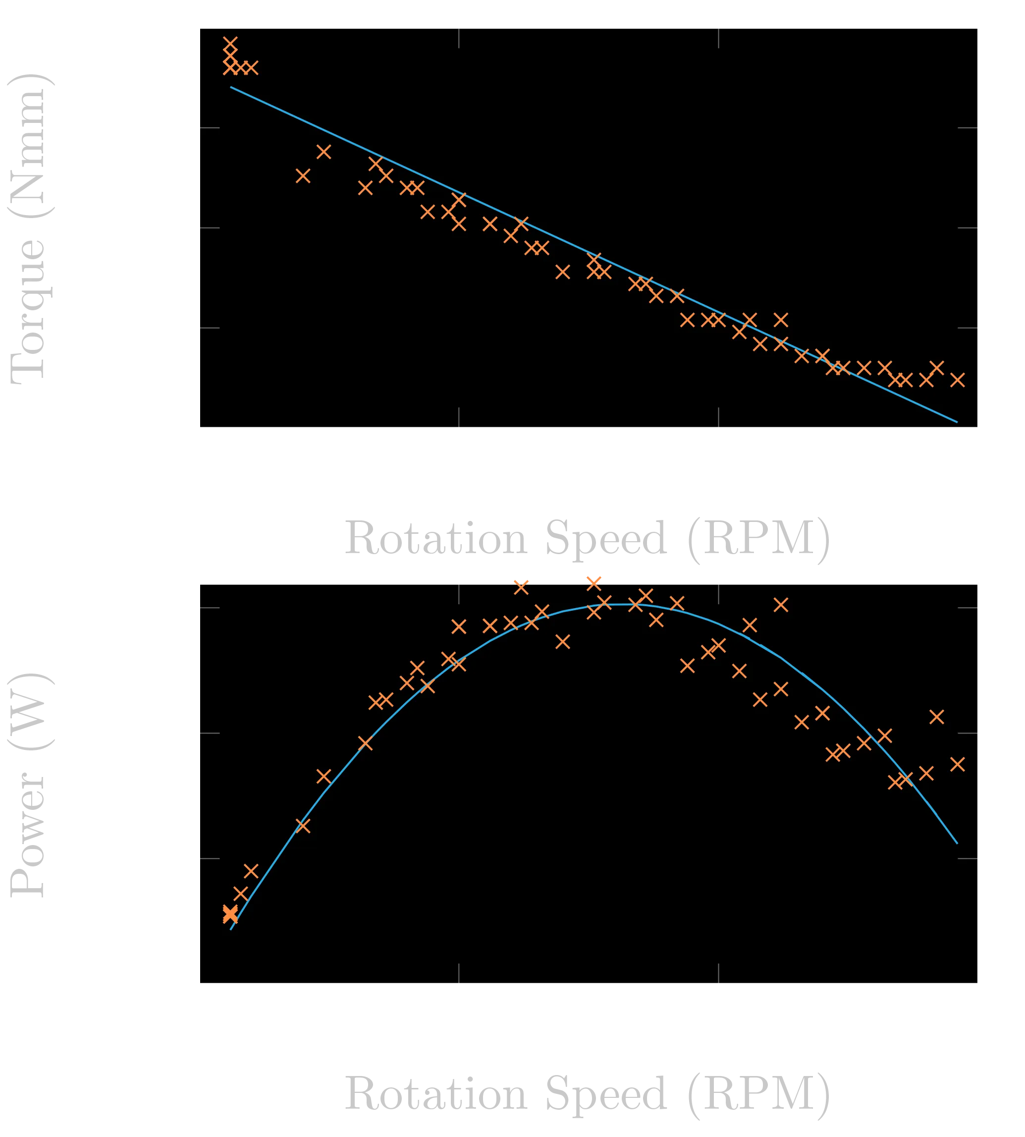
We tested the dynamometer using another DC motor purchased from a local shop. The dynamometer was connected to a computer so the results could be plotted in real time. The measurement results are shown in Figure 18.

Conclusions

In this project, an electric absorption dynamometer was designed, modeled, and built. It successfully measured a motor’s power at different speeds.

First, different types of dynamometers were researched, and their fundamental principles were analyzed. The absorption unit was selected to be a DC generator. After selecting the absorption method, the dynamometer was carefully formulated, and the required components were selected and designed to meet the project goals. The system was then modeled mathematically to ensure the components met the design criteria. A MATLAB code was developed to simulate the dynamometer and was made available on GitHub. Finally, the dynamometer was assembled, and the electronic circuit was designed and programmed.

Ideas for the Future

Potential improvements for future development include:

1. Controlling the load electronically by replacing the potentiometer with a digital potentiometer or using another motor to adjust it.
2. Using higher-precision sensors for more accurate measurements.
3. Measuring torque and back EMF constants with high-precision instruments to improve reliability.
4. Reusing the generator’s output power for useful work instead of dissipating it as heat.

Notes

1. Willard W. Pulkrabek. Engineering Fundamentals of the Internal Combustion Engine. Prentice Hall, 1997. ISBN 9780135708545. ↩

2. MatthiasDD. Schematic of a prony brake. URL: https://commons.wikimedia.org/wiki/File:Prony_brake.svg (visited on 2022-05-07). ↩

3. JohnnyQ90. Simplest dyno for rc engines! - prony brake dynamometer!. URL: https://youtu.be/0ESOYhOh28c (visited on 2022-05-19). ↩

4. Raymond A. Serway and Jr. John W. Jewett. Physics for Scientists and Engineers with Modern Physics. Cengage Learning, 2014. ISBN 9781133954057. ↩ ↩² ↩³

5. Chetvorno. Eddy current brake diagram. URL: https://en.wikipedia.org/wiki/File:Eddy_current_brake_diagram.svg (visited on 2022-05-07). ↩

6. Nagwa. Lesson explainer: direct current motors. URL: https://www.nagwa.com/en/explainers/246108560531 (visited on 2022-05-08). ↩

7. Norman S. Nise. Control Systems Engineering. Wiley, 2019. ISBN 9781119474210. ↩ ↩²

8. James W. Nilsson and Susan A. Riedel. Electric Circuits. Pearson Education, 2014. ISBN 9780133594812. ↩

9. Ivo Leito, Lauri Jalukse, and Irja Helm. Estimation of measurement uncertainty in chemical analysis (analytical chemistry) course. 2020. URL: https://sisu.ut.ee/measurement/uncertainty. ↩

10. PJRC. Teensy 3.2 development board. URL: https://www.pjrc.com/store/teensy32.html (visited on 2023-01-08). ↩